Consider a finite population of \(N\) animals. Similarly to the
motivating example for replicator dynamics, these animals when they interact will
always share their food. Due to a genetic mutation, some of these animals may
act in an aggressive manner and not share their food. If two aggressive animals
meet they both compete and end up with no food. If an aggressive animal meets a
sharing one, the aggressive one will take most of the food.
The difference with a replicator dynamics model is that it will be assumed that
the size of the population is finite and stays constant.
These interactions can be represented using the matrix
\(A\):
In this scenario: what is the probability that the mutation takes over the
entire population?
To answer this question we will assume a vector \(v\) represents the
population. In this case:
\(v_1\) represents the number of individuals of the population that share.
\(v_2\) represents the number of individuals of the population that act aggressively.
Note that as the size of the population is assumed to be constant this implies
that:
\[\sum_i x_i = N\]
Where \(N\) is the number of individuals in the population.
The overall fitness of an individual of a given type in a population \(v\)
is then given by the expected utility (as given by \(A\)) of individuals of
that type as they interact with the population:
The evolutionary process defined in this chapter will assume an individual will
be selected for copy proportional to their fitness. The probability of picking
an individual of a given type \(i\) is thus given by:
\[\frac{v_i f_i}{v_1 f_1 + v_2 f_2}\]
To ensure the population stays constant this requires that an individual is
chosen to be removed. This is done uniformly randomly. The probability of
picking an individual of a given type \(i\) for removal is then given by:
\[\frac{v_i}{v_1 + v_2}\]
These probabilities allow us to define a Markov process that describes
the evolution of the system. Here is a diagram showing the different states in
the process for \(N=5\).
        stateDiagram-v2
    direction LR
    s1: (1, 4)
    s2: (2, 3)
    s3: (3, 2)
    s4: (4, 1)

    s1 --> s2
    s2 --> s1

    s2 --> s3
    s3 --> s2

    s3 --> s4
    s4 --> s3

    note left of s1
        (0, 5)
    end note

    note right of s4
        (5, 0)
    end note
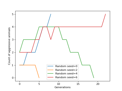
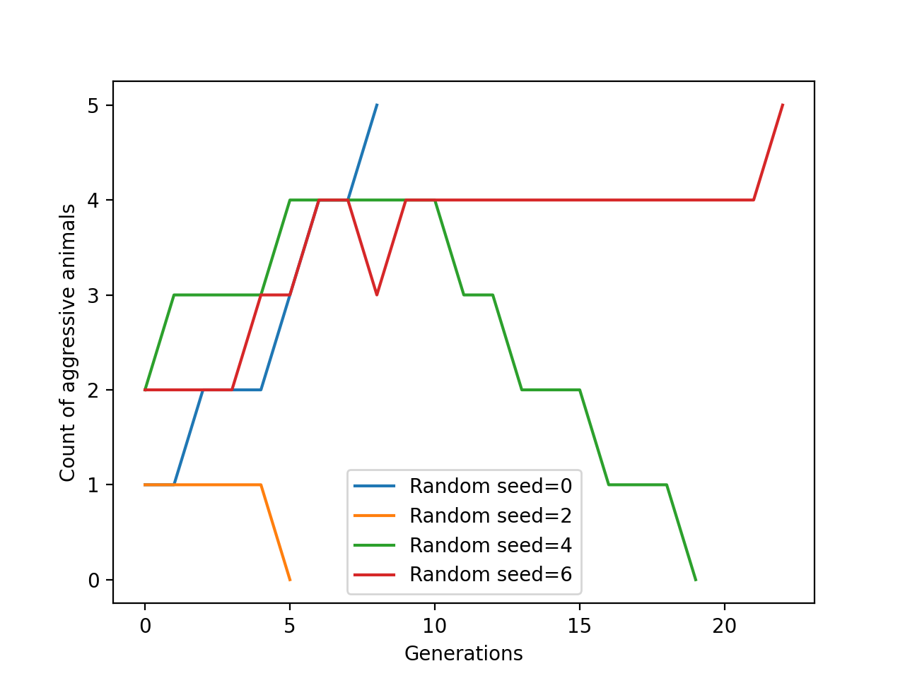
The answer to our question corresponds to the probability that starting in state
\(v=(4, 1)\), we arrive at state \(v=(0, 5)\).
The following plot shows 4 possible outcomes. In 2 of them the sharing animals
resist the invasion of the aggressive one.
First defined in [Moran1958] the Moran process assumes a constant population of
\(N\) individuals which can be of \(m\) different types. There exists a
fitness function \(f:[1, \dots, m] \times [1, \dots, m] ^ N \to \mathbb{R}\)
that maps each individual to a numeric fitness value which is dependent on the
types of the individuals in the population.
The process is defined as follows, at each step:
Every individual \(k\) has their fitness \(f_k\) calculated.
An individual is randomly selected for copying. This selection is done
proportional to their fitness: \(f_k(v)\). Thus, the probability of selecting
individual \(k\) for copying is given by:
\[\frac{f_k(v)}{\sum_{h=1^N}f_h(v)}\]
An individual is selected for removal. This selection is done uniformly
randomly. Thus, the probability of selecting individual \(i\) for removal
is given by:
\[1 / N\]
An individual of the same type as the individual selected for copying is
introduced to the population.
The individual selected for removal is removed.
The process is repeated until there is only one type of individual left in the
population.
A common representation of the fitness function \(f\) is to use a game.
As an example consider a population with \(N=10\) and \(m=3\) types of
individuals. The fitness of a given individual is calculated by considering the
utilities received by each individual when they interact with all other
individuals. These interactions are given by the \(3\times 3\) matrix
\(A\):
The Moran process can be modified to allow for mutation. When a new individual
is selected for copying, there is a \(p\) probability that they mutate to a
another type from the original population (even if they are no longer present in
the population.
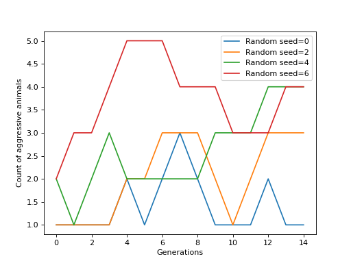
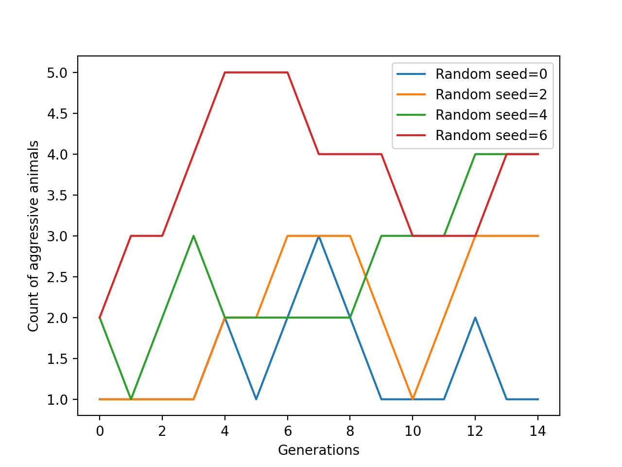
The following plot shows 4 possible outcomes of the Moran process of the
Hawk Dove game with a probability of
mutation of \(p=.2\). Note that as opposed to the numerical simulations
without mutation, the process does not terminate as new types of individuals can
always enter the population.
When considering a Moran process on 2 types of individuals the fitness function
is defined by
\(A\) which is, in this case is a 2 by 2 matrix.
In the case of a only two types of individuals, the population vector \(v\)
can be replaced by an integer \(n\) which represents the number of
individuals of the first type. The number of individuals of the second type is
then given by \(N - n\).
In this case the random process is a specific type of process called a birth
death process:
A set of possible states: \(S = \{0, 1, \dots, N\}\)
Two absorbing states: \(0\) and N.
Probabilities \(p_{ij}\) of going from state \(i\) to \(j\)
defined by:
\(p_{i, i + 1} + p_{i, i - 1} \leq 1\) for \(1\leq i \leq N - 1\).
\(p_{ii} = 1 - p_{i, i + 1} - p_{i, i - 1}\) for \(1\leq i \leq N - 1\).
For the following games, obtain the fixation probability \(x_1\)
for \(N=4\):
\(A=\begin{pmatrix}1 & 1 \\ 1 & 1\end{pmatrix}\)
\(A=\begin{pmatrix}1 & 2 \\ 3 & 1\end{pmatrix}\)
Consider the game
\(A=\begin{pmatrix}r & 1 \\ 1 & 1\end{pmatrix}\) for \(r>1\)
and \(N\), and obtain \(x_1\) as a function of \(r\). How
does \(r\) effect the chance of fixation?
Prove the theorem for fixation probabilities in a birth
death process (a Moran process with 2 types).
See Use Moran processes for guidance of how to use Nashpy to obtain
numerical simulations of the Moran process. See
Obtain fixation probabilities for guidance of how to use Nashpy to
obtain approximations of the fixation probabilities. This is what is used to
obtain all the plots above.


