Discrete Replicator dynamics

Motivating example: once a day hawk dove game

Consider the Hawk Dove model shown in replicator dynamics, where we wish to model the populations of aggressive and sharing animals over time but assume the population of aggressive and sharing animals only changes once a day.

We use the following payoff matrix:

\[\begin{split}A = \begin{pmatrix} 2 & 1\\ 3 & 0 \end{pmatrix}\end{split}\]

and starting population distribution

\[\begin{split}x_0 = \begin{pmatrix}0.05\\0.95\end{pmatrix}\end{split}\]

where 95% are sharers while 5% are aggressive.

How would we model this situation with the added constraint of discrete time?

The discrete replicator dynamics equation

Given a population with \(N\) types of individuals. Where the fitness of an individual of type \(i\) when interacting with an individual of type \(j\) is given by \(A_{ij}\) where \(A\in\mathbb{R}^{N \times N}\). The discrete replicator dynamics equation defines a sequence \(x^{(t)}\) given by:

\[x_{i}^{(t + 1)} = x_i^{(t)} \frac{(Ax)_i}{{x^{(t)}}^T A x^{(t)}}\]

where:

\[\phi = \sum_{i=1} ^ N x_i^{(t)} f_i(x)\]

where \(f_i\) is the population dependent fitness of individuals of type \(i\):

\[f_i(x) = (Ax^{(t)})_i\]

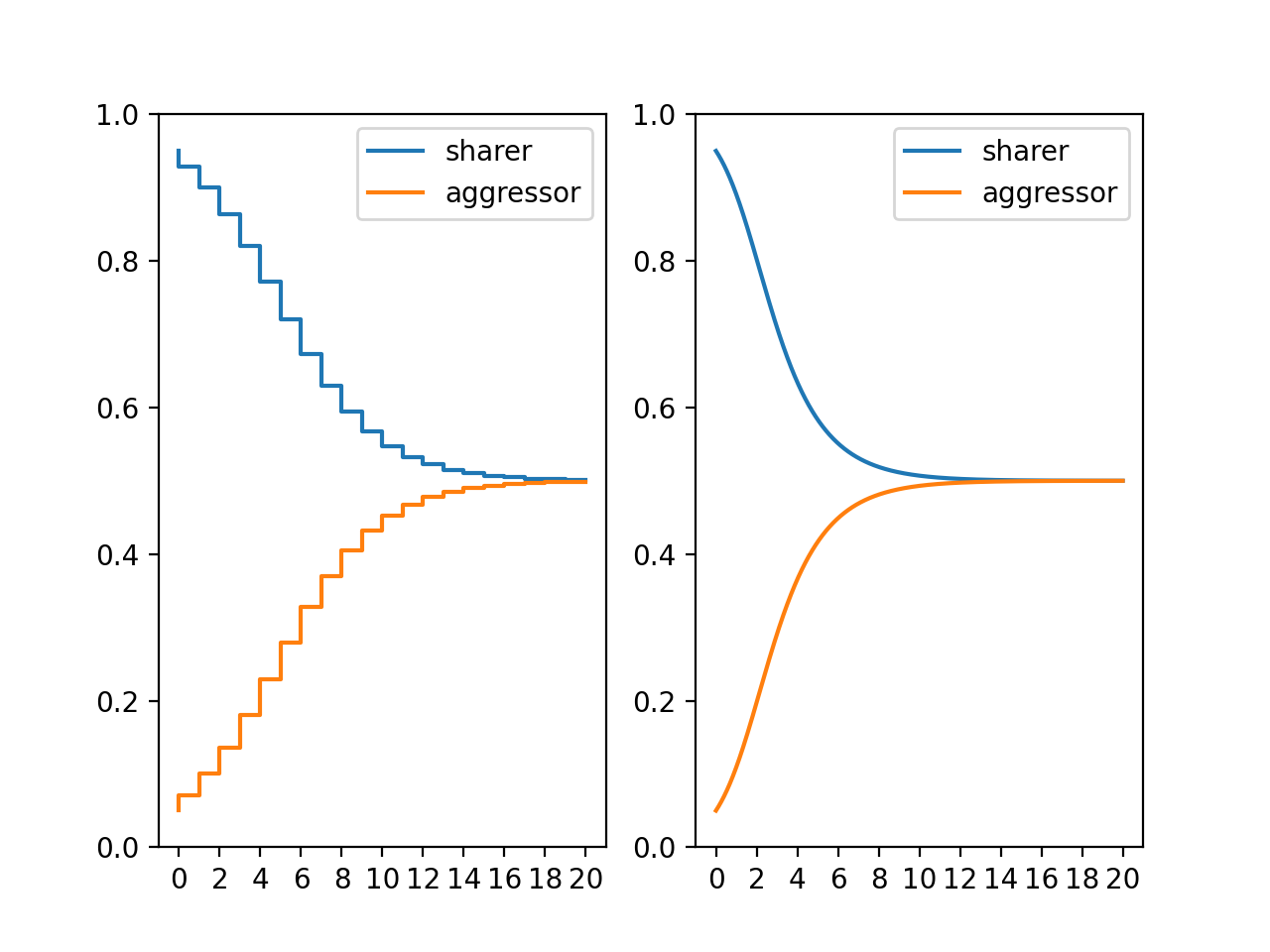
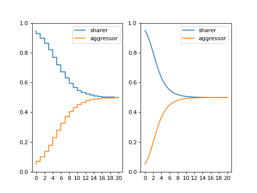
For the Motivating example: once a day hawk dove game this gives discrete results (on the left) similar to the continuous replicator function (on the right).

(Source code, png, hires.png, pdf)

Both the continuous and discrete replicator functions produce a proportion of a total population, this addresses the first modelling challenge: to have discrete time.

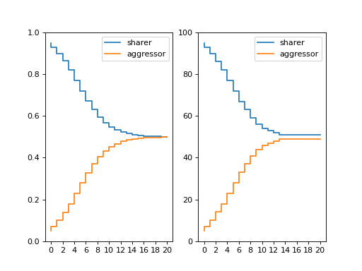
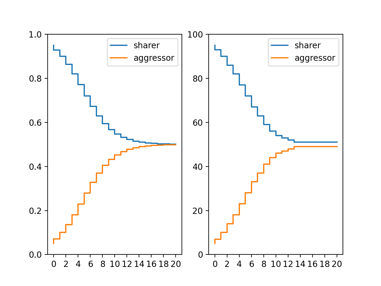
However what if we wanted to model a finite population of 100 animals?

Quantizing a Population Distribution

This algorithm is first described in [Greenwood2019], the aim is to convert a continuous population distribution \(\mathbf{x} = (x_1, \dots, x_n)\) into a vector of integer counts \(\mathbf{k} = (k_1, \dots, k_n)\) such that the entries sum exactly to \(N\) while remaining as close as possible to the unquantised values \(N x_i\).

This quantization step is done at every step of the discrete replicator dynamics to ensure the population vector remains integer.

Algorithm (Quantisation of a Population Distribution)

Given a population distribution \(\mathbf{x}\) and a total population \(N\), proceed as follows:

1. Initial rounding step

   For each \(i = 1, \dots, n\), compute

   \[k'_i = \left\lfloor N x_i - \tfrac{1}{2} \right\rfloor.\]

2. Check population consistency

   Compute the discrepancy

   \[d = \sum_{i=1}^n k'_i - N.\]

   If \(d = 0\), return \(\mathbf{k}'\) immediately.

3. Compute rounding errors

   For each \(i\), compute the error

   \[\delta_i = k'_i - N x_i,\]

   which quantifies the deviation of \(k'_i\) from its exact value \(N x_i\).

4. Adjust to restore the correct total

   • If \(d > 0\) (too many individuals have been allocated):

     Select the \(d\) largest errors \(\delta_i\) and decrement each corresponding \(k'_i\) by 1.

   • If \(d < 0\) (too few individuals have been allocated):

     Select the \(|d|\) smallest errors \(\delta_i\) and increment each corresponding \(k'_i\) by 1.

5. Return the corrected population

   The adjusted vector \(\mathbf{k}'\) now sums to \(N\) and is the closest integer-valued approximation to the unquantised population \(N \mathbf{x}\).

(Source code, png, hires.png, pdf)

Using Nashpy

See Use discrete replicator dynamics for guidance of how to use Nashpy to obtain numerical solutions of the discrete replicator dynamics equation.